Getting-started tutorial No. 1: Liquid methanol
In this tutorial, we train ML dipole models of liquid methanol and calculate the dipole moments along the MD trajectory.
Required data for calculations
To train ML models for dipole moment, we only need two files:
atomic coordinates with Wannier centers
molecular structure (chemical bond information)
The first file is assumed to be the extended xyz format via ase package, which also contains the supercell information. The second file should be a standard mol file to be processed using rdkit. We prepared a simple example using the isolated methanol system for this tutorial. Necessary files are included in this repository. Let’s go to tutorial/tutorial1/.
$cd examples/tutorial/1_liquidmethanol/
$tree
├── IONS+CENTERS+cell_sorted_merge.xyz -> ../../CPtrain/cptrain_train/IONS+CENTERS+cell_sorted_merge.xyz
├── config.yaml
├── methanol.mol
└── train.yaml
xyz format atomic structures for training data
The order of atoms should satisfy three things
The atomic order must be molecule-by-molecule.
The atomic order in each molecule should be the same as the
*.molfile.The WCs should come last.
If you see the first 8 lines of methanol.xyz, you can find C, four H, and O. The Wannier centers (WC) are represented as X. There are the atoms and WCs included in a single MD step.
$ cat methanol.xyz
416
Lattice="12.911606431431386 0.0 0.0 0.0 12.911606431431386 0.0 0.0 0.0 12.911606431431386" Properties=species:S:1:pos:R:3 pbc="T T T"
C       10.70302493      10.85955260       8.68064224
O        9.72875172      10.09124538       9.38880112
H       10.70478669      10.62022413       7.61094586
H       11.69788485      10.69544339       9.10099246
H       10.46045016      11.94347292       8.76860487
H        9.43087091      10.68001118      10.11893151
They are visualized using nglview package via jupyter notebook as follows.
%pip install nglview
%pip install ase
        import nglview as nv
        import ase.io

# read all the trajectory.
# If you want to extract a single step instead, try like ase.io.read("filename", index=1)
        aseatoms = ase.io.read("mol_wan.xyz",index=":")

# This if for list of ase.atoms. If you want to see single ase.atom, use nv.show_ase.
        w = nv.show_asetraj(aseatoms,gui=True)
        w.clear_representations()
        w.add_label(radius=0.2,color="black",label_type="atom")
        w.add_ball_and_stick("_He",color="green",radius=0.004,aspectRatio=50)
        w.add_ball_and_stick("_Ne",color="cyan",radius=0.004,aspectRatio=50)
        w.add_ball_and_stick("_Ar",color="green",radius=0.004,aspectRatio=50)
        #w.add_ball_and_stick("_Li",color="cyan",radius=0.1)
        #w.add_ball_and_stick("_Be",color="blue",radius=0.1)
        w.add_ball_and_stick("_H")
        w.add_ball_and_stick("_C")
        w.add_ball_and_stick("_O")
        w.add_ball_and_stick("_N")

        w.add_unitcell()
        w.update_unitcell()
        w
We have 10000 MD steps in the file, which will be used for both training and validation data for ML.
# see how many steps in the aseatoms
print(len(aseatoms))
Mol file for bond information
Next, we dig into the *.mol file, which contains molecular structures including atomic and bonding information.
$ cat methanol.mol
6  5  0  0  0  0  0  0  0  0999 V2000
    0.9400    0.0200   -0.0900 C   0  0  0  0  0  0  0  0  0  0  0  0
    0.4700    0.2700   -1.4000 O   0  0  0  0  0  0  0  0  0  0  0  0
    0.5800   -0.9500    0.2400 H   0  0  0  0  0  0  0  0  0  0  0  0
    0.5700    0.8000    0.5800 H   0  0  0  0  0  0  0  0  0  0  0  0
    2.0400    0.0200   -0.0900 H   0  0  0  0  0  0  0  0  0  0  0  0
    0.8100    1.1400   -1.6700 H   0  0  0  0  0  0  0  0  0  0  0  0
1  5  1  0  0  0  0
1  3  1  0  0  0  0
1  4  1  0  0  0  0
2  1  1  0  0  0  0
6  2  1  0  0  0  0
M  END
The second to seventh lines are called atom block, which contain atomic coordinates and species in a single molecule. We only use atomic species for training. The following data is called atom block, representing bonding information.
1 5 1 0 0 0 0
For example, the above line means the first and fifth atom (C and H) have a chemical bond. In other words, the atoms with first two numbers have a chemical bond. The *.mol format is a standard format for molecular structures, and you can easily find information on it.
Model training
Prepare input parameters
To train models, we implemented CPtrain.py command written in python. The command requires a yaml format file to specify parameters. Here is an example:
model:
modelname:
    - ch  # specify name
    - oh
    - o
    - co
nfeature:  288   # length of descriptor
M:         20    # M  (embedding matrix size)
Mb:        6     # Mb (embedding matrix size, smaller than M)

learning_rate:
type: fix

loss:
type: mse        # mean square error

data:
type: xyz        # or xyz
file:
    - "IONS+CENTERS+cell_sorted_merge.xyz"
itp_file: methanol.mol
bond_name:
    - CH
    - OH
    - O
    - CO
bondtype:
    - CH_1_bond
    - OH_1_bond
    - Olp
    - CO_1_bond

training:
device:     cpu # Torchのdevice
batch_size: 32  # batch size for training
validation_batch_size: 32 # batch size for validation
max_epochs: 50
learning_rate:
    type: ExponentialLR
    start_lr: 1e-3 # starting learning rate
    gamma: 0.95
n_train:     900    # the number of training data (frame)
n_val:       100    # the number of validation data (frame)
modeldir:
    - model_ch # directory to save models
    - model_oh
    - model_o
    - model_co
restart:   False    # If restart training
Parameters written above are basically necessary values (not optional). The input file consists of four parts:
part name |
explanation |
|---|---|
model |
ML model parameters |
learning_rate |
learning rate |
loss |
loss function |
data |
training data |
training |
training parameters |
As Basic explanations are given above, we only add some important notes.
model
Model parameters (
nfeature,M,Mb) given above are basically enough for simple gas/liquid molecules. Although the detailed meanings of the parameters will be given later, we emphasize thatMbshould be smaller thanMby definition, and that nfeature should be a multiple of4.modelnameis just used for file names, so you can use any word as you like.
learning_rate
Currently, we only support fixed learning rate.
loss
Currently, We only support Mean Squared Error (MSE) as a loss function.
data
Training data should be
descriptororxyz. In this tutorial, we usexyztype.If training data type is
descriptor, the descriptor file name should be*_descs.npy, and the true file name should be*_true.npy.bondtypedefines which bond to be trained. The value is one ofCH,CO,OH,CC, orO.To train models for all the chemical bond species, We list the all chemical bond species in
bondtype.
training
deviceis the same aspytorch’s device for model training. You can use cpu, cuda, or mps.modeldirspecifies the directory to which model files will be saved.
Train a model
After the training script is prepared, we can start the training by simply running
CPtrain.py train -i train.yaml
The code generates stdout like
your python version is ...  3 11

*****************************************************************
                    CPtrain.py
                    Version. 0.0.1
*****************************************************************

2024-05-27 23:21:32,907 root mltrain [INFO]: Start logging
{'model': {'modelname': 'test', 'nfeature': 288, 'M': 20, 'Mb': 6}, 'learning_rate': {'type': 'fix'}, 'loss': {'type': 'mse'}, 'data': {'type': 'xyz', 'file': ['IONS+CENTERS+cell_sorted_merge.xyz'], 'itp_file': 'methanol.mol'}, 'training': {'device': 'cpu', 'batch_size': 32, 'validation_batch_size': 32, 'max_epochs': 40, 'learning_rate': '1e-2', 'n_train': 900, 'n_val': 100, 'modeldir': 'model_test', 'restart': False}}
model NET :: nfeatures ::  288
nfeatures_enet :: 72
nfeatures_fnet :: 120
=================================================================
Layer (type:depth-idx)                   Param #
=================================================================
NET_withoutBN                            --
├─Linear: 1-1                            3,650
├─Linear: 1-2                            2,550
├─Linear: 1-3                            73,440
├─Linear: 1-4                            6,050
├─Linear: 1-5                            2,550
├─Linear: 1-6                            1,020
=================================================================
Total params: 89,260
Trainable params: 89,260
Non-trainable params: 0
=================================================================
2024-05-27 23:21:32,927 root mltrain [INFO]:  --------------------------------------
data type :: xyz
-----  ml.read_mol :: parse results... -------
bonds_list ::  [[0, 4], [0, 2], [0, 3], [1, 0], [5, 1]]
counter    ::  6
atom_list  ::  ['C', 'O', 'H', 'H', 'H', 'H']
-----------------------------------------------
================
CH bonds...       [[0, 4], [0, 2], [0, 3]]
CO bonds...       [[1, 0]]
OH bonds...       [[5, 1]]
OO bonds...       []
CC bonds...       []
CC ring bonds...  []


==================
ring_bond_index  []
ch_bond_index    [0, 1, 2]
oh_bond_index    [4]
co_bond_index    [3]
cc_bond_index    []
================
O atoms (lonepair)...       [1]
N atoms (lonepair)...       []
C atoms ...                 [0]
H atoms ...                 [2, 3, 4, 5]
C 0.94 0.02 -0.09
O 0.47 0.27 -1.4
-----  ml.read_mol :: parse results... -------
representative_atom_index  :: 1
-----------------------------------------------
================
coh_index/coc_index :: [oの番号, {coボンドの番号(co_bond_indexの0から数えていくつか),ohボンドの番号}]
TODO :: もしかしたらbond_indexを使った方が全体的にやりやすいかもしれない
coh_index :: [[0, {'CO': 0, 'OH': 0}]]
coc_index :: []
Loading xyz file ::  ['IONS+CENTERS+cell_sorted_merge.xyz']
len xyz == 1
2024-05-27 23:21:34,561 root mltrain [INFO]:  -----------------------------------------------------------------
2024-05-27 23:21:34,561 root mltrain [INFO]:  ---Summary of DataSystem: training     ----------------------------------
2024-05-27 23:21:34,561 root mltrain [INFO]: found 1 system(s):
2024-05-27 23:21:34,561 root mltrain [INFO]:                         system  natoms  bch_sz   n_bch
2024-05-27 23:21:34,561 root mltrain [INFO]: IONS+CENTERS+cell_sorted_merge.xyz    1000      32      31
2024-05-27 23:21:34,562 root mltrain [INFO]: --------------------------------------------------------------------------------------
splitting atoms into atoms and WCs
Assigning Wannier Centers
Finish Assigning Wannier Centers
2024-05-27 23:22:28,891 Trainer __init__ [INFO]: model data will be saved to model_test
=================================================================
Layer (type:depth-idx)                   Param #
=================================================================
NET_withoutBN                            --
├─Linear: 1-1                            3,650
├─Linear: 1-2                            2,550
├─Linear: 1-3                            73,440
├─Linear: 1-4                            6,050
├─Linear: 1-5                            2,550
├─Linear: 1-6                            1,020
=================================================================
Total params: 89,260
Trainable params: 89,260
Non-trainable params: 0
=================================================================

2024-05-27 23:22:28,892 Trainer init_model [INFO]: Torch device (cpu or cuda gpu or m1 mac gpu): cpu
2024-05-27 23:22:29,384 numexpr.utils _init_num_threads [INFO]: Note: NumExpr detected 16 cores but "NUMEXPR_MAX_THREADS" not set, so enforcing safe limit of 8.
2024-05-27 23:22:29,384 numexpr.utils _init_num_threads [INFO]: NumExpr defaulting to 8 threads.
2024-05-27 23:22:29,556 Trainer set_dataset [INFO]:  n_traing ( number of training  data): 900
2024-05-27 23:22:29,556 Trainer set_dataset [INFO]:  n_val    ( number of validatin data): 100
^@2024-05-27 23:23:05,110 Trainer epoch_step [INFO]: epoch= 1 : time= 35.553799867630005 [s] : loss(train)= 0.0030520600183600827 : loss(valid)= 0.0028606270595143237 : RMSE[D](train)= 0.0551564542987999 : RMSE[D](valid)= 0.05347409362915805
model is saved to model_test_tmp1.pt at model_test
2024-05-27 23:23:41,283 Trainer epoch_step [INFO]: epoch= 2 : time= 36.05292296409607 [s] : loss(train)= 0.002742534619756043 : loss(valid)= 0.002425628947094083 : RMSE[D](train)= 0.05222889056766713 : RMSE[D](valid)= 0.04924118021059818
model is saved to model_test_tmp2.pt at model_test
2024-05-27 23:24:17,498 Trainer epoch_step [INFO]: epoch= 3 : time= 36.17855882644653 [s] : loss(train)= 0.0027552477217146327 : loss(valid)= 0.0023257903133829436 : RMSE[D](train)= 0.05240615377016262 : RMSE[D](valid)= 0.04821778239842708
model is saved to model_test_tmp3.pt at model_test
2024-05-27 23:24:52,931 Trainer epoch_step [INFO]: epoch= 4 : time= 35.389596939086914 [s] : loss(train)= 0.002701992983929813 : loss(valid)= 0.002566932700574398 : RMSE[D](train)= 0.051863416078856424 : RMSE[D](valid)= 0.0505809825728987
model is saved to model_test_tmp4.pt at model_test
2024-05-27 23:25:28,712 Trainer epoch_step [INFO]: epoch= 5 : time= 35.72677397727966 [s] : loss(train)= 0.0026170784757206483 : loss(valid)= 0.0026297084211061397 : RMSE[D](train)= 0.05109348549317842 : RMSE[D](valid)= 0.05118794610165333
model is saved to model_test_tmp5.pt at model_test
2024-05-27 23:26:02,858 Trainer epoch_step [INFO]: epoch= 6 : time= 34.10452723503113 [s] : loss(train)= 0.002519122832122126 : loss(valid)= 0.002710235926012198 : RMSE[D](train)= 0.05010292158956631 : RMSE[D](valid)= 0.05182654546680134
model is saved to model_test_tmp6.pt at model_test
2024-05-27 23:26:36,344 Trainer epoch_step [INFO]: epoch= 7 : time= 33.43118190765381 [s] : loss(train)= 0.002488897938746959 : loss(valid)= 0.002438249376912912 : RMSE[D](train)= 0.04980324078916386 : RMSE[D](valid)= 0.04936132032714493
model is saved to model_test_tmp7.pt at model_test
2024-05-27 23:27:09,524 Trainer epoch_step [INFO]: epoch= 8 : time= 33.13404870033264 [s] : loss(train)= 0.0024281473555934747 : loss(valid)= 0.0024121985770761967 : RMSE[D](train)= 0.049172273966610065 : RMSE[D](valid)= 0.04911379181779723
model is saved to model_test_tmp8.pt at model_test
2024-05-27 23:27:42,988 Trainer epoch_step [INFO]: epoch= 9 : time= 33.424768924713135 [s] : loss(train)= 0.0024187416752933393 : loss(valid)= 0.00232696447831889 : RMSE[D](train)= 0.04911207242387859 : RMSE[D](valid)= 0.04820846097177897
model is saved to model_test_tmp9.pt at model_test
2024-05-27 23:28:17,375 Trainer epoch_step [INFO]: epoch= 10 : time= 34.339770793914795 [s] : loss(train)= 0.002027994516538456 : loss(valid)= 0.0020500118068108955 : RMSE[D](train)= 0.04497044101939407 : RMSE[D](valid)= 0.045273193022861896
model is saved to model_test_tmp10.pt at model_test
2024-05-27 23:28:50,388 Trainer epoch_step [INFO]: epoch= 11 : time= 32.96853709220886 [s] : loss(train)= 0.0018060718056014074 : loss(valid)= 0.0015387694584205747 : RMSE[D](train)= 0.042402016109021445 : RMSE[D](valid)= 0.0391866800126098
model is saved to model_test_tmp11.pt at model_test
2024-05-27 23:29:23,494 Trainer epoch_step [INFO]: epoch= 12 : time= 33.06202292442322 [s] : loss(train)= 0.0015744604378206922 : loss(valid)= 0.001602462415272991 : RMSE[D](train)= 0.03961410282709073 : RMSE[D](valid)= 0.03996957523043282
model is saved to model_test_tmp12.pt at model_test
2024-05-27 23:29:56,833 Trainer epoch_step [INFO]: epoch= 13 : time= 33.296122789382935 [s] : loss(train)= 0.0015049170885634208 : loss(valid)= 0.0015406373422592878 : RMSE[D](train)= 0.03872750117829672 : RMSE[D](valid)= 0.039230152528586505
model is saved to model_test_tmp13.pt at model_test
2024-05-27 23:30:30,009 Trainer epoch_step [INFO]: epoch= 14 : time= 33.13048601150513 [s] : loss(train)= 0.0014625149363252734 : loss(valid)= 0.0013872180522109072 : RMSE[D](train)= 0.038211363274244604 : RMSE[D](valid)= 0.03717074105946483
model is saved to model_test_tmp14.pt at model_test
2024-05-27 23:31:03,023 Trainer epoch_step [INFO]: epoch= 15 : time= 32.970470905303955 [s] : loss(train)= 0.0012952481338288635 : loss(valid)= 0.0011708201685299475 : RMSE[D](train)= 0.03594431862161766 : RMSE[D](valid)= 0.034191540839132055
model is saved to model_test_tmp15.pt at model_test
2024-05-27 23:31:37,101 Trainer epoch_step [INFO]: epoch= 16 : time= 34.034749031066895 [s] : loss(train)= 0.0012781490970935141 : loss(valid)= 0.0012487516505643725 : RMSE[D](train)= 0.03567568660112371 : RMSE[D](valid)= 0.03530874235402812
model is saved to model_test_tmp16.pt at model_test
2024-05-27 23:32:10,323 Trainer epoch_step [INFO]: epoch= 17 : time= 33.178393840789795 [s] : loss(train)= 0.0012396411870473198 : loss(valid)= 0.0012016038332755368 : RMSE[D](train)= 0.0351610294889353 : RMSE[D](valid)= 0.0346635038703976
model is saved to model_test_tmp17.pt at model_test
2024-05-27 23:32:43,535 Trainer epoch_step [INFO]: epoch= 18 : time= 33.16394877433777 [s] : loss(train)= 0.0012235958503359662 : loss(valid)= 0.0012918139109387994 : RMSE[D](train)= 0.03492190754501672 : RMSE[D](valid)= 0.03592647573961546
model is saved to model_test_tmp18.pt at model_test
2024-05-27 23:33:16,961 Trainer epoch_step [INFO]: epoch= 19 : time= 33.37561392784119 [s] : loss(train)= 0.0012278797990542703 : loss(valid)= 0.0012458103786533077 : RMSE[D](train)= 0.03499613492118348 : RMSE[D](valid)= 0.035192720360356027
model is saved to model_test_tmp19.pt at model_test
2024-05-27 23:33:50,577 Trainer epoch_step [INFO]: epoch= 20 : time= 33.57127404212952 [s] : loss(train)= 0.0012240493794836635 : loss(valid)= 0.001295727367202441 : RMSE[D](train)= 0.03495633493656875 : RMSE[D](valid)= 0.03591999197134574
model is saved to model_test_tmp20.pt at model_test
2024-05-27 23:34:23,622 Trainer epoch_step [INFO]: epoch= 21 : time= 32.997060775756836 [s] : loss(train)= 0.0012256120015600963 : loss(valid)= 0.0011909629683941603 : RMSE[D](train)= 0.03495001219865892 : RMSE[D](valid)= 0.03448448842303
model is saved to model_test_tmp21.pt at model_test
2024-05-27 23:34:56,853 Trainer epoch_step [INFO]: epoch= 22 : time= 33.18896174430847 [s] : loss(train)= 0.0012167344518404985 : loss(valid)= 0.0012835346860811114 : RMSE[D](train)= 0.034833311084896894 : RMSE[D](valid)= 0.03577993540008407
model is saved to model_test_tmp22.pt at model_test
2024-05-27 23:35:29,807 Trainer epoch_step [INFO]: epoch= 23 : time= 32.91186189651489 [s] : loss(train)= 0.0011236058489885181 : loss(valid)= 0.0011108355053390067 : RMSE[D](train)= 0.03343205283435263 : RMSE[D](valid)= 0.03328191643945063
model is saved to model_test_tmp23.pt at model_test
2024-05-27 23:36:03,022 Trainer epoch_step [INFO]: epoch= 24 : time= 33.170867919921875 [s] : loss(train)= 0.001198199895692856 : loss(valid)= 0.0011316734598949552 : RMSE[D](train)= 0.03454902092721321 : RMSE[D](valid)= 0.03361872941420203
model is saved to model_test_tmp24.pt at model_test
2024-05-27 23:36:36,357 Trainer epoch_step [INFO]: epoch= 25 : time= 33.290594816207886 [s] : loss(train)= 0.0011569774401972868 : loss(valid)= 0.00125562238584583 : RMSE[D](train)= 0.03398148767577144 : RMSE[D](valid)= 0.03526287444169499
model is saved to model_test_tmp25.pt at model_test
2024-05-27 23:37:09,678 Trainer epoch_step [INFO]: epoch= 26 : time= 33.2756552696228 [s] : loss(train)= 0.0010826434694796003 : loss(valid)= 0.0012303667608648539 : RMSE[D](train)= 0.03285225680652831 : RMSE[D](valid)= 0.0350027180085837
model is saved to model_test_tmp26.pt at model_test
2024-05-27 23:37:43,053 Trainer epoch_step [INFO]: epoch= 27 : time= 33.32958698272705 [s] : loss(train)= 0.001173686479367981 : loss(valid)= 0.0010828875432101388 : RMSE[D](train)= 0.034169700120643916 : RMSE[D](valid)= 0.03287867522535803
model is saved to model_test_tmp27.pt at model_test
2024-05-27 23:38:19,747 Trainer epoch_step [INFO]: epoch= 28 : time= 36.647231101989746 [s] : loss(train)= 0.001116036980030393 : loss(valid)= 0.0012196329965566595 : RMSE[D](train)= 0.03330824263660591 : RMSE[D](valid)= 0.03489144527681723
model is saved to model_test_tmp28.pt at model_test
2024-05-27 23:38:59,670 Trainer epoch_step [INFO]: epoch= 29 : time= 39.88249492645264 [s] : loss(train)= 0.0011180073737965099 : loss(valid)= 0.0012258108084400494 : RMSE[D](train)= 0.03336500989034002 : RMSE[D](valid)= 0.03500258438073604
model is saved to model_test_tmp29.pt at model_test
2024-05-27 23:39:49,398 Trainer epoch_step [INFO]: epoch= 30 : time= 49.675516843795776 [s] : loss(train)= 0.0010629503813106567 : loss(valid)= 0.0010745280305854976 : RMSE[D](train)= 0.03253391709756107 : RMSE[D](valid)= 0.03270917398237465
model is saved to model_test_tmp30.pt at model_test
2024-05-27 23:40:26,195 Trainer epoch_step [INFO]: epoch= 31 : time= 36.73529386520386 [s] : loss(train)= 0.0010963863585077757 : loss(valid)= 0.001109493294886003 : RMSE[D](train)= 0.03305228076125506 : RMSE[D](valid)= 0.03320700290457949
model is saved to model_test_tmp31.pt at model_test
2024-05-27 23:41:06,045 Trainer epoch_step [INFO]: epoch= 32 : time= 39.80792784690857 [s] : loss(train)= 0.001064531773278889 : loss(valid)= 0.0011376045683088403 : RMSE[D](train)= 0.032547290130018745 : RMSE[D](valid)= 0.03362633110102043
model is saved to model_test_tmp32.pt at model_test
2024-05-27 23:41:46,186 Trainer epoch_step [INFO]: epoch= 33 : time= 40.091362953186035 [s] : loss(train)= 0.0010355500500216813 : loss(valid)= 0.0009315957043630382 : RMSE[D](train)= 0.03212837784581807 : RMSE[D](valid)= 0.030487922940679202
model is saved to model_test_tmp33.pt at model_test
2024-05-27 23:42:21,759 Trainer epoch_step [INFO]: epoch= 34 : time= 35.53277611732483 [s] : loss(train)= 0.0009523128766366946 : loss(valid)= 0.0008897289323310057 : RMSE[D](train)= 0.030749915142596514 : RMSE[D](valid)= 0.029788555875735753
model is saved to model_test_tmp34.pt at model_test
2024-05-27 23:42:57,443 Trainer epoch_step [INFO]: epoch= 35 : time= 35.59277606010437 [s] : loss(train)= 0.0009194710645325748 : loss(valid)= 0.0008036431002741059 : RMSE[D](train)= 0.030231966427741203 : RMSE[D](valid)= 0.028328095215842314
model is saved to model_test_tmp35.pt at model_test
2024-05-27 23:43:34,729 Trainer epoch_step [INFO]: epoch= 36 : time= 37.2429301738739 [s] : loss(train)= 0.0008694644493516535 : loss(valid)= 0.0008589115265446404 : RMSE[D](train)= 0.02939380869049454 : RMSE[D](valid)= 0.029268487767904347
model is saved to model_test_tmp36.pt at model_test
2024-05-27 23:44:10,015 Trainer epoch_step [INFO]: epoch= 37 : time= 35.23839807510376 [s] : loss(train)= 0.0008100573946389236 : loss(valid)= 0.0007349376101046801 : RMSE[D](train)= 0.02839690322675918 : RMSE[D](valid)= 0.0270813759830895
model is saved to model_test_tmp37.pt at model_test
2024-05-27 23:44:46,935 Trainer epoch_step [INFO]: epoch= 38 : time= 36.876343965530396 [s] : loss(train)= 0.0008246830173967672 : loss(valid)= 0.0007781900543098649 : RMSE[D](train)= 0.028661926251427983 : RMSE[D](valid)= 0.027891913603732336
model is saved to model_test_tmp38.pt at model_test
2024-05-27 23:45:27,108 Trainer epoch_step [INFO]: epoch= 39 : time= 40.12124514579773 [s] : loss(train)= 0.0008413328593763124 : loss(valid)= 0.0008210245287045836 : RMSE[D](train)= 0.028899934585797222 : RMSE[D](valid)= 0.02863102027700547
model is saved to model_test_tmp39.pt at model_test
2024-05-27 23:46:17,073 Trainer epoch_step [INFO]: epoch= 40 : time= 49.92154312133789 [s] : loss(train)= 0.0008217944268835708 : loss(valid)= 0.0008133725496008992 : RMSE[D](train)= 0.028557669288744897 : RMSE[D](valid)= 0.028495248694122847
model is saved to model_test_tmp40.pt at model_test
model is saved to model_test_weight.pth at model_test
model is saved to model_test_all.pth at model_test
model is saved to model_test.pt at model_test
Test a model
We can check the quality of the trained model using a yaml structure file.
The trained model is stored in the directory specified by modeldir and the seed in the training input file.
In our case, the model is saved in model_ch_seed_42/model_ch.pt. We can test the trained model by running
CPtrain.py test -m model_ch_seed_42/model_ch.pt -x IONS+CENTERS+cell_sorted_merge.xyz -i methanol.mol
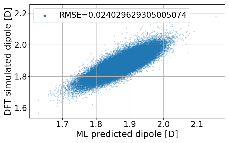
It takes a few minutes to complete the calculation. The code generates two figures and two text files. The figures are the correlation between the predicted and true dipole moments (and the absolute value of the dipole moment). The text files named pred_list.txt and true_list.txt contain the predicted dipole moments and the true dipole moments, and they are visualized in pred_true_norm.png and pred_true_density.png.
Calculate dipoles along MD trajectories (Python interface)
After constructing four dipole moment models (CH, CO, OH, and O) and validating our trained model works well, we try our model on molecular dynamics trajectories using Python interface.
Here we use the pre-trained models we prepared, which are stored in model_rotate_methanol/. You can also train your own model and use it for the following calculation.
Let’s first move to the example directory.
cd examples/CPtrain/cptrain_pred_v3
The input file for the Python code is given in yaml format and is as follows.
general:
    bondfilename: methanol.mol
    savedir: dipole_10ps/
    temperature: 300
    timestep: 0.484
descriptor:
    calc: 1
    directory: ./
    xyzfilename: IONS+CENTERS+cell_sorted_merge.xyz
    savedir: dipole_10ps/
    descmode: 2
    desctype: allinone
    haswannier: 1
    interval: 1
    desc_coh: 0
    Rcs: 4
    Rc: 6
predict:
    calc: 1
    desc_dir: dipole_10ps/
    model_dir: model_met/
    device: cpu
    modelmode: rotate
    bondspecies: 4
    save_truey: 0
The input composes of three part, general, descriptor, and predict. The details of the parameters are given bellow.
general
bondfilename[required]:
molfile for the molecule. (methanol in our case)savedir[required]: The directory to which all the outputs will be saved.
temperature[optional]: We can optionally set the temperature to calculate dielectric properties. The default is 300 [Kelvin]
timestep[optional]: We can optionally set the MD timestep to calculate dynamical dielectric properties.
descriptor
calc[required]: 1 for doing calculation, 0 for skip calculation.
directory[required]: The directory in which the input xyz is stored.
xyzfilename[required]: The input xyz filename.
desctype[required]: The type of descriptor. Currently we have
allinoneandold.
- predict:
calc: 1
desc_dir: dipole_10ps/
model_dir: model_met/
modelmode: rotate
bondspecies: 4
save_truey: 0
The calculation is performed by running the following command.
CPtrain.py pred -i config.yaml
After the calculation, the following result files are saved in the directory specified by savedir.
total_dipole.txt: system total dipole.mol_wan.xyz: atomic and predicted WCs configurations inxyzformat.DIELCONST: dielectric constant and average molecular dipole.
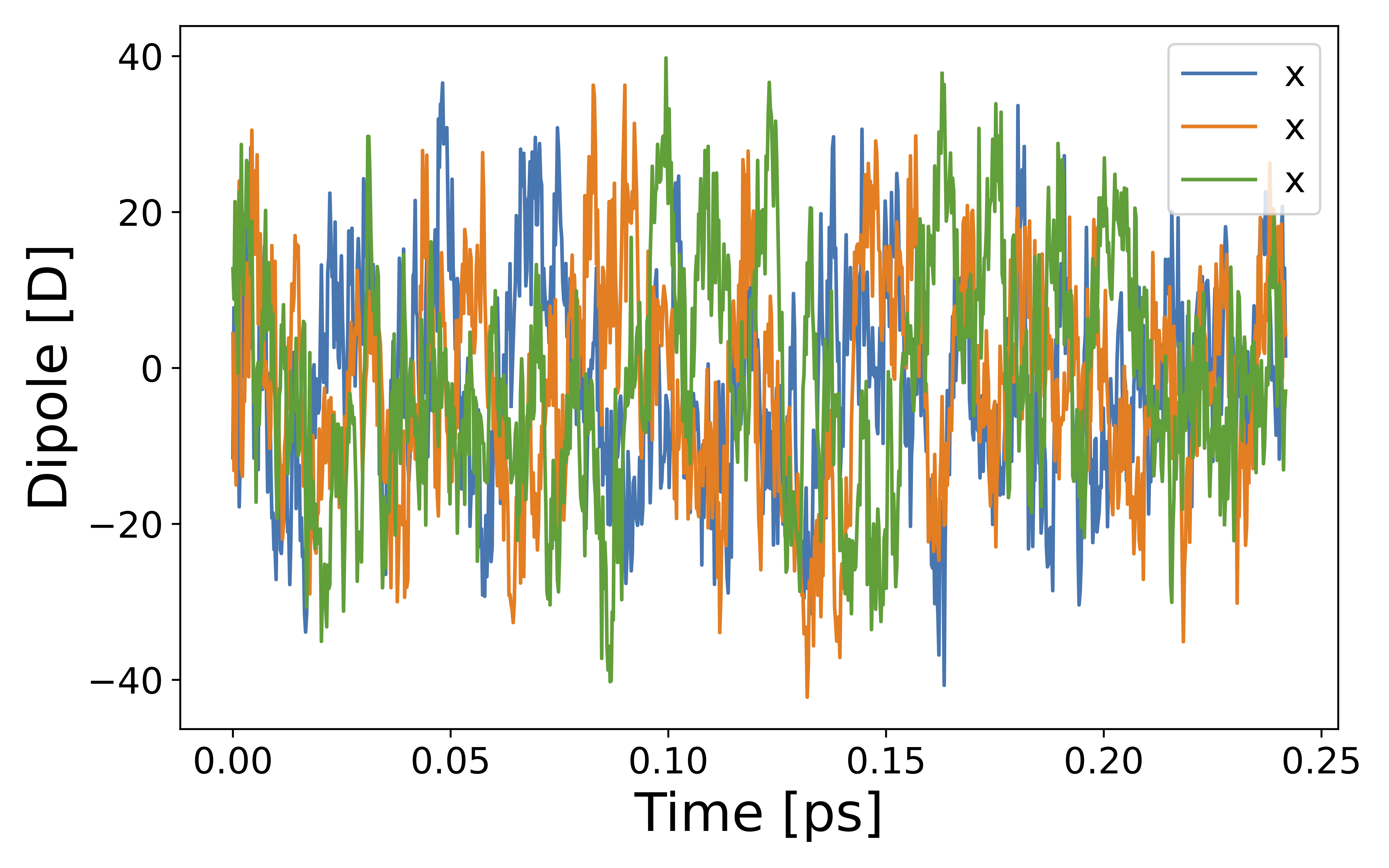
We can visualize the system dipole moment along the MD trajectory using total_dipole.txt to see if our calculation success.
CPextract.py diel total -F dipole_10ps/total_dipole.txt
Finally, we perform Fourier transformation of the total dipole moments to calculate the dielectric function via CPextract.py command. You must specify the high-frequency dielectric constant with -E option
CPextract.py diel spectra -F total_dipole.txt -E 1.76624 -s 0 -w 1
The above command generate three files:
total_dipole.txt_diel.csv: real and imaginary parts of the dielectric function.total_dipole.txt_refractive.csv: real and imaginary parts of the complex refractive index.total_dipole.txt_alphan.csv: absorption spectraalpha(\omega)*n(\omega).
Here we visualize the imaginary part of the dielectric function using the following python script.
import matplotlib as mpl
import matplotlib.pyplot as plt
import numpy as np
import pandas as pd
# load data
df = pd.read_csv("dipole_10ps/total_dipole.txt_diel.csv")

# figure instantce
fig, ax = plt.subplots(figsize=(8,5),tight_layout=True)
ax.plot(df["freq_kayser"], df["imag_diel"],label="imag_diel",lw=3)
ax.set_xlim(0,3500)
#
xticklabels = ax.get_xticklabels()
yticklabels = ax.get_yticklabels()
xlabel="Frequency [cm-1]"
ylabel="Epsilon"

#
ax.set_xlabel(xlabel,fontsize=22)
ax.set_ylabel(ylabel,fontsize=22)
ax.grid()
ax.tick_params(axis='x', labelsize=20 )
ax.tick_params(axis='y', labelsize=20 )
lgnd=ax.legend(loc="upper left",fontsize=20)
# lgnd.legendHandles[0]._sizes = [30]
# lgnd.legendHandles[0]._alpha = [1.0]
fig.savefig("imag_diel.png")
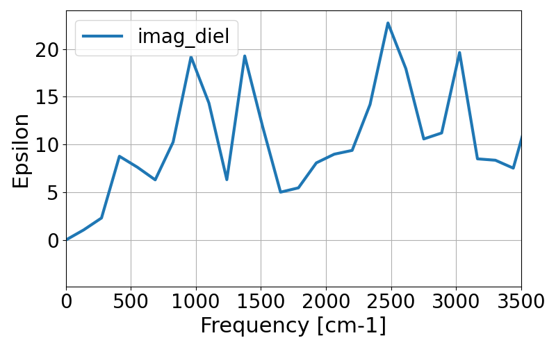
As the MD trajectory is too short, we can not get meaningful spectra. We will acquire better one in the following tutorials.
Calculate dipoles along MD trajectories (C++ interface)
After constructing four dipole moment models (CH, CO, OH, and O) and validating our trained model works well, we try our model on molecular dynamics trajectories using C++ interface. Let us go to the example directory
cd examples/dieltools/methanol
The input file for the C++ code is given in yaml format and is as follows.
general:
    itpfilename: methanol.acpype/input_GMX.mol
    bondfilename: methanol.mol
    savedir: dipole_10ps/
    temperature: 300
    timestep: 0.242
descriptor:
    calc: 1
    directory: ./
    xyzfilename: IONS+CENTERS+cell_sorted_merge.xyz
    savedir: dipole_10ps/
    descmode: 2
    desctype: allinone
    haswannier: 1   # if WCs are in xyz, set 1
    interval: 1
    desc_coh: 0
predict:
    calc: 1
    desc_dir: dipole_10ps/
    model_dir: model_rotate_methanol/
    modelmode: rotate
    bondspecies: 4
    save_truey: 0
The input composes of three part, general, descripter, and predict. The details of the parameters are given bellow.
general
itpfilename[required]:
molfile for the molecule. (methanol in our case)savedir[required]: The directory to which all the outputs will be saved.
temperature[optional]: We can optionally set the temperature to calculate dielectric properties. The default is 300 [Kelvin]
timestep[optional]: We can optionally set the MD timestep to calculate dynamical dielectric properties.
descripter
calc[required]: 1 for doing calculation, 0 for skip calculation.
directory[required]: The directory in which the input xyz is stored.
xyzfilename[required]: The input xyz filename.
desctype[required]: The type of descriptor. Currently we have
allinoneandold.
- predict:
calc: 1
desc_dir: dipole_10ps/
model_dir: /home/k0151/k015124/c++/20231025_model_rotate_methanol/
modelmode: rotate
bondspecies: 4
save_truey: 0
You can perform C++ calculations with enabling OpenMP. For example, you can set the number of threads to 12 by running
export OMP_NUM_THREADS=12
dieltools config.yaml
After the calculation, the following result files are saved in the directory specified by savedir.
total_dipole.txt: system total dipole.mol_wan.xyz: atomic and predicted WCs configurations inxyzformat.DIELCONST: dielectric constant and average molecular dipole.
We can visualize the system dipole moment along the MD trajectory using total_dipole.txt to see if our calculation success.
CPextract.py diel total -F dipole_10ps/total_dipole.txt

Finally, we perform Fourier transformation of the total dipole moments to calculate the dielectric function via CPextract.py command. You must specify the high-frequency dielectric constant with -E option
CPextract.py diel spectra -F total_dipole.txt -E 1.76624 -s 0 -w 1
The above command generate three files:
total_dipole.txt_diel.csv: real and imaginary parts of the dielectric function.total_dipole.txt_refractive.csv: real and imaginary parts of the complex refractive index.total_dipole.txt_alphan.csv: absorption spectraalpha(\omega)*n(\omega).
Here we visualize the imaginary part of the dielectric function using the following python script.
import matplotlib as mpl
import matplotlib.pyplot as plt
import numpy as np
import pandas as pd
# load data
df = pd.read_csv("dipole_10ps/total_dipole.txt_diel.csv")

# figure instantce
fig, ax = plt.subplots(figsize=(8,5),tight_layout=True)
ax.plot(df["freq_kayser"], df["imag_diel"],label="imag_diel",lw=3)
ax.set_xlim(0,3500)
#
xticklabels = ax.get_xticklabels()
yticklabels = ax.get_yticklabels()
xlabel="Frequency [cm-1]"
ylabel="Epsilon"

#
ax.set_xlabel(xlabel,fontsize=22)
ax.set_ylabel(ylabel,fontsize=22)
ax.grid()
ax.tick_params(axis='x', labelsize=20 )
ax.tick_params(axis='y', labelsize=20 )
lgnd=ax.legend(loc="upper left",fontsize=20)
# lgnd.legendHandles[0]._sizes = [30]
# lgnd.legendHandles[0]._alpha = [1.0]
fig.savefig("imag_diel.png")

As the MD trajectory is too short, we can not get meaningful spectra. We will acquire better one in the following tutorials.